Business Statistics B.B.A.LLB 1st sem Notes

 

 

 

Created By Shubham Yadav

 

Meet me on Insta

 

SUBJECT: BUSINESS STATISTICS  

 

AN INTRODUCTION TO BUSINESS STATISTICS 

OBJECTIVE: The aim of the present lesson is to enable the students to understand  the meaning, definition, nature, importance and limitations of statistics.  

Kya karoge padke kiska bhala hua hai, Lol

“A knowledge of statistics is like a knowledge of foreign 

language of algebra; it may prove of use at any time under  

any circumstance”……………………………………...Bowley.  

STRUCTURE:  

1.1 Introduction  

1.2 Meaning and Definitions of Statistics  

1.3 Types of Data and Data Sources  

1.4 Types of Statistics  

1.5 Scope of Statistics  

1.6 Importance of Statistics in Business  

1.7 Limitations of statistics  

1.8 Summary  

1.9 Self-Test Questions  

1.10 Surprise

1.1 INTRODUCTION  

For a layman, ‘Statistics’ means numerical information expressed in quantitative  terms. This information may relate to objects, subjects, activities, phenomena, or  regions of space. As a matter of fact, data have no limits as to their reference,  coverage, and scope. At the macro level, these are data on gross national product and  shares of agriculture, manufacturing, and services in GDP (Gross Domestic Product).  

1 

At the micro level, individual firms, howsoever small or large, produce extensive  statistics on their operations. The annual reports of companies contain variety of data  on sales, production, expenditure, inventories, capital employed, and other activities.  These data are often field data, collected by employing scientific survey techniques.  Unless regularly updated, such data are the product of a one-time effort and have  limited use beyond the situation that may have called for their collection. A student  knows statistics more intimately as a subject of study like economics, mathematics,  chemistry, physics, and others. It is a discipline, which scientifically deals with data,  and is often described as the science of data. In dealing with statistics as data,  statistics has developed appropriate methods of collecting, presenting, summarizing,  and analysing data, and thus consists of a body of these methods.  

          1.2 MEANING AND DEFINITIONS OF STATISTICS  

            In the beginning, it may be noted that the word ‘statistics’ is used rather curiously in  two senses plural and singular. In the plural sense, it refers to a set of figures or data.  In the singular sense, statistics refers to the whole body of tools that are used to  collect data, organise and interpret them and, finally, to draw conclusions from them.  It should be noted that both the aspects of statistics are important if the quantitative  data are to serve their purpose. If statistics, as a subject, is inadequate and consists of  poor methodology, we could not know the right procedure to extract from the data the  information they contain. Similarly, if our data are defective or that they are  inadequate or inaccurate, we could not reach the right conclusions even though our  subject is well developed.  

A.L. Bowley has defined statistics as: (i) statistics is the science of counting, (ii)  Statistics may rightly be called the science of averages, and (iii) statistics is the  science of measurement of social organism regarded as a whole in all its mani-

2 

festations. Boddington defined as: Statistics is the science of estimates and  probabilities. Further, W.I. King has defined Statistics in a wider context, the science  of Statistics is the method of judging collective, natural or social phenomena from the  results obtained by the analysis or enumeration or collection of estimates.  

Seligman explored that statistics is a science that deals with the methods of collecting,  classifying, presenting, comparing and interpreting numerical data collected to throw  some light on any sphere of enquiry. Spiegal defines statistics highlighting its role in  decision-making particularly under uncertainty, as follows: statistics is concerned  with scientific method for collecting, organising, summa rising, presenting and  analyzing data as well as drawing valid conclusions and making reasonable decisions  on the basis of such analysis. According to Prof. Horace Secrist, Statistics is the  aggregate of facts, affected to a marked extent by multiplicity of causes, numerically  expressed, enumerated or estimated according to reasonable standards of accuracy,  collected in a systematic manner for a pre-determined purpose, and placed in relation  to each other.  

From the above definitions, we can highlight the major characteristics of statistics as  follows:  

(i) Statistics are the aggregates of facts. It means a single figure is not statistics.  For example, national income of a country for a single year is not statistics but  the same for two or more years is statistics.  

(ii) Statistics are affected by a number of factors. For example, sale of a product  depends on a number of factors such as its price, quality, competition, the  income of the consumers, and so on. 

3 

(iii) Statistics must be reasonably accurate. Wrong figures, if analysed, will lead to  erroneous conclusions. Hence, it is necessary that conclusions must be based  on accurate figures.  

(iv) Statistics must be collected in a systematic manner. If data are collected in a  haphazard manner, they will not be reliable and will lead to misleading  conclusions.  

(v) Collected in a systematic manner for a pre-determined purpose  (vi) Lastly, Statistics should be placed in relation to each other. If one collects data  unrelated to each other, then such data will be confusing and will not lead to  any logical conclusions. Data should be comparable over time and over space.  1.3 TYPES OF DATA AND DATA SOURCES  

Statistical data are the basic raw material of statistics. Data may relate to an activity of  our interest, a phenomenon, or a problem situation under study. They derive as a  result of the process of measuring, counting and/or observing. Statistical data,  therefore, refer to those aspects of a problem situation that can be measured,  quantified, counted, or classified. Any object subject phenomenon, or activity that  generates data through this process is termed as a variable. In other words, a variable  is one that shows a degree of variability when successive measurements are recorded.  In statistics, data are classified into two broad categories: quantitative data and  qualitative data. This classification is based on the kind of characteristics that are  measured.  

Quantitative data are those that can be quantified in definite units of measurement.  These refer to characteristics whose successive measurements yield quantifiable  observations. Depending on the nature of the variable observed for measurement,  quantitative data can be further categorized as continuous and discrete data. 

4 

Obviously, a variable may be a continuous variable or a discrete variable.  (i) Continuous data represent the numerical values of a continuous variable. A  continuous variable is the one that can assume any value between any two  points on a line segment, thus representing an interval of values. The values  are quite precise and close to each other, yet distinguishably different. All  characteristics such as weight, length, height, thickness, velocity, temperature,  tensile strength, etc., represent continuous variables. Thus, the data recorded  on these and similar other characteristics are called continuous data. It may be  noted that a continuous variable assumes the finest unit of measurement.  Finest in the sense that it enables measurements to the maximum degree of  precision.  

(ii) Discrete data are the values assumed by a discrete variable. A discrete  variable is the one whose outcomes are measured in fixed numbers. Such data  are essentially count data. These are derived from a process of counting, such  as the number of items possessing or not possessing a certain characteristic.  The number of customers visiting a departmental store everyday, the incoming  flights at an airport, and the defective items in a consignment received for sale,  are all examples of discrete data.  

Qualitative data refer to qualitative characteristics of a subject or an object. A  characteristic is qualitative in nature when its observations are defined and noted in  terms of the presence or absence of a certain attribute in discrete numbers. These data  are further classified as nominal and rank data.  

(i) Nominal data are the outcome of classification into two or more categories of  items or units comprising a sample or a population according to some quality  characteristic. Classification of students according to sex (as males and 

5 

females), of workers according to skill (as skilled, semi-skilled, and unskilled),  and of employees according to the level of education (as matriculates,  undergraduates, and post-graduates), all result into nominal data. Given any  such basis of classification, it is always possible to assign each item to a  particular class and make a summation of items belonging to each class. The  count data so obtained are called nominal data.  

(ii) Rank data, on the other hand, are the result of assigning ranks to specify order  in terms of the integers 1,2,3, ..., n. Ranks may be assigned according to the  level of performance in a test. a contest, a competition, an interview, or a  show. The candidates appearing in an interview, for example, may be assigned  ranks in integers ranging from I to n, depending on their performance in the  interview. Ranks so assigned can be viewed as the continuous values of a  variable involving performance as the quality characteristic.  

Data sources could be seen as of two types, viz., secondary and primary. The two can  be defined as under:  

(i) Secondary data: They already exist in some form: published or unpublished -  in an identifiable secondary source. They are, generally, available from  published source(s), though not necessarily in the form actually required.  

(ii) Primary data: Those data which do not already exist in any form, and thus  have to be collected for the first time from the primary source(s). By their very  nature, these data require fresh and first-time collection covering the whole  population or a sample drawn from it.  

1.4 TYPES OF STATISTICS  

There are two major divisions of statistics such as descriptive statistics and inferential  statistics. The term descriptive statistics deals with collecting, summarizing, and 

6 

simplifying data, which are otherwise quite unwieldy and voluminous. It seeks to  achieve this in a manner that meaningful conclusions can be readily drawn from the  data. Descriptive statistics may thus be seen as comprising methods of bringing out  and highlighting the latent characteristics present in a set of numerical data. It not  only facilitates an understanding of the data and systematic reporting thereof in a  manner; and also makes them amenable to further discussion, analysis, and  interpretations.  

The first step in any scientific inquiry is to collect data relevant to the problem in  hand. When the inquiry relates to physical and/or biological sciences, data collection  is normally an integral part of the experiment itself. In fact, the very manner in which  an experiment is designed, determines the kind of data it would require and/or  generate. The problem of identifying the nature and the kind of the relevant data is  thus automatically resolved as soon as the design of experiment is finalized. It is  possible in the case of physical sciences. In the case of social sciences, where the  required data are often collected through a questionnaire from a number of carefully  selected respondents, the problem is not that simply resolved. For one thing,  designing the questionnaire itself is a critical initial problem. For another, the number  of respondents to be accessed for data collection and the criteria for selecting them  has their own implications and importance for the quality of results obtained. Further,  the data have been collected, these are assembled, organized, and presented in the  form of appropriate tables to make them readable. Wherever needed, figures,  diagrams, charts, and graphs are also used for better presentation of the data. A useful  tabular and graphic presentation of data will require that the raw data be properly  classified in accordance with the objectives of investigation and the relational analysis  to be carried out. . 

7 

A well thought-out and sharp data classification facilitates easy description of the  hidden data characteristics by means of a variety of summary measures. These include  measures of central tendency, dispersion, skewness, and kurtosis, which constitute the  essential scope of descriptive statistics. These form a large part of the subject matter  of any basic textbook on the subject, and thus they are being discussed in that order  here as well.  

Inferential statistics, also known as inductive statistics, goes beyond describing a  given problem situation by means of collecting, summarizing, and meaningfully  presenting the related data. Instead, it consists of methods that are used for drawing  inferences, or making broad generalizations, about a totality of observations on the  basis of knowledge about a part of that totality. The totality of observations about  which an inference may be drawn, or a generalization made, is called a population or  a universe. The part of totality, which is observed for data collection and analysis to  gain knowledge about the population, is called a sample.  

The desired information about a given population of our interest; may also be  collected even by observing all the units comprising the population. This total  coverage is called census. Getting the desired value for the population through census  is not always feasible and practical for various reasons. Apart from time and money  considerations making the census operations prohibitive, observing each individual  unit of the population with reference to any data characteristic may at times involve  even destructive testing. In such cases, obviously, the only recourse available is to  employ the partial or incomplete information gathered through a sample for the  purpose. This is precisely what inferential statistics does. Thus, obtaining a particular  value from the sample information and using it for drawing an inference about the  entire population underlies the subject matter of inferential statistics. Consider a 

8 

situation in which one is required to know the average body weight of all the college  students in a given cosmopolitan city during a certain year. A quick and easy way to  do this is to record the weight of only 500 students, from out of a total strength of,  say, 10000, or an unknown total strength, take the average, and use this average based  on incomplete weight data to represent the average body weight of all the college  students. In a different situation, one may have to repeat this exercise for some future  year and use the quick estimate of average body weight for a comparison. This may  be needed, for example, to decide whether the weight of the college students has  undergone a significant change over the years compared.  

Inferential statistics helps to evaluate the risks involved in reaching inferences or  generalizations about an unknown population on the basis of sample information. for  example, an inspection of a sample of five battery cells drawn from a given lot may  reveal that all the five cells are in perfectly good condition. This information may be  used to conclude that the entire lot is good enough to buy or not.  

Since this inference is based on the examination of a sample of limited number of  cells, it is equally likely that all the cells in the lot are not in order. It is also possible  that all the items that may be included in the sample are unsatisfactory. This may be  used to conclude that the entire lot is of unsatisfactory quality, whereas the fact may  indeed be otherwise. It may, thus, be noticed that there is always a risk of an inference  about a population being incorrect when based on the knowledge of a limited sample.  The rescue in such situations lies in evaluating such risks. For this, statistics provides  the necessary methods. These centres on quantifying in probabilistic term the chances  of decisions taken on the basis of sample information being incorrect. This requires an  understanding of the what, why, and how of probability and probability distributions  to equip ourselves with methods of drawing statistical inferences and estimating the 

9 

degree of reliability of these inferences.  

1.5 SCOPE OF STATISTICS 

Apart from the methods comprising the scope of descriptive and inferential branches  of statistics, statistics also consists of methods of dealing with a few other issues of  specific nature. Since these methods are essentially descriptive in nature, they have  been discussed here as part of the descriptive statistics. These are mainly concerned  with the following:  

(i) It often becomes necessary to examine how two paired data sets are related.  For example, we may have data on the sales of a product and the expenditure  incurred on its advertisement for a specified number of years. Given that sales  and advertisement expenditure are related to each other, it is useful to examine  the nature of relationship between the two and quantify the degree of that  relationship. As this requires use of appropriate statistical methods, these falls  under the purview of what we call regression and correlation analysis.  

(ii) Situations occur quite often when we require averaging (or totalling) of data  on prices and/or quantities expressed in different units of measurement. For  example, price of cloth may be quoted per meter of length and that of wheat  per kilogram of weight. Since ordinary methods of totalling and averaging do  not apply to such price/quantity data, special techniques needed for the  purpose are developed under index numbers.  

(iii) Many a time, it becomes necessary to examine the past performance of an  activity with a view to determining its future behaviour. For example, when  engaged in the production of a commodity, monthly product sales are an  important measure of evaluating performance. This requires compilation and  analysis of relevant sales data over time. The more complex the activity, the 

10 

more varied the data requirements. For profit maximising and future sales  planning, forecast of likely sales growth rate is crucial. This needs careful  collection and analysis of past sales data. All such concerns are taken care of  under time series analysis.  

(iv) Obtaining the most likely future estimates on any aspect(s) relating to a  business or economic activity has indeed been engaging the minds of all  concerned. This is particularly important when it relates to product sales and  demand, which serve the necessary basis of production scheduling and  planning. The regression, correlation, and time series analyses together help  develop the basic methodology to do the needful. Thus, the study of methods  and techniques of obtaining the likely estimates on business/economic  variables comprises the scope of what we do under business forecasting.  

Keeping in view the importance of inferential statistics, the scope of statistics may  finally be restated as consisting of statistical methods which facilitate decision-- making under conditions of uncertainty. While the term statistical methods is often  used to cover the subject of statistics as a whole, in particular it refers to methods by  which statistical data are analysed, interpreted, and the inferences drawn for decision making.  

Though generic in nature and versatile in their applications, statistical methods have  come to be widely used, especially in all matters concerning business and economics.  These are also being increasingly used in biology, medicine, agriculture, psychology,  and education. The scope of application of these methods has started opening and  expanding in a number of social science disciplines as well. Even a political scientist  finds them of increasing relevance for examining the political behaviour and it is, of  course, no surprise to find even historians statistical data, for history is essentially past 

11 

data presented in certain actual format.  

1.6 IMPORTANCE OF STATISTICS IN BUSINESS  

There are three major functions in any business enterprise in which the statistical  methods are useful. These are as follows:  

(i) The planning of operations: This may relate to either special projects or to  the recurring activities of a firm over a specified period.  

(ii) The setting up of standards: This may relate to the size of employment,  volume of sales, fixation of quality norms for the manufactured product,  norms for the daily output, and so forth.  

(iii) The function of control: This involves comparison of actual production  achieved against the norm or target set earlier. In case the production has  fallen short of the target, it gives remedial measures so that such a deficiency  does not occur again.  

A worth noting point is that although these three functions-planning of operations,  setting standards, and control-are separate, but in practice they are very much  interrelated.  

Different authors have highlighted the importance of Statistics in business. For  instance, Croxton and Cowden give numerous uses of Statistics in business such as  project planning, budgetary planning and control, inventory planning and control,  quality control, marketing, production and personnel administration. Within these also  they have specified certain areas where Statistics is very relevant. Another author,  Irwing W. Burr, dealing with the place of statistics in an industrial organisation,  specifies a number of areas where statistics is extremely useful. These are: customer  wants and market research, development design and specification, purchasing, 

12 

production, inspection, packaging and shipping, sales and complaints, inventory and  maintenance, costs, management control, industrial engineering and research.  Statistical problems arising in the course of business operations are multitudinous. As  such, one may do no more than highlight some of the more important ones to  emphasis the relevance of statistics to the business world. In the sphere of production,  for example, statistics can be useful in various ways.  

Statistical quality control methods are used to ensure the production of quality goods.  Identifying and rejecting defective or substandard goods achieve this. The sale targets  can be fixed on the basis of sale forecasts, which are done by using varying methods  of forecasting. Analysis of sales affected against the targets set earlier would indicate  the deficiency in achievement, which may be on account of several causes: (i) targets  were too high and unrealistic (ii) salesmen's performance has been poor (iii)  emergence of increase in competition (iv) poor quality of company's product, and so  on. These factors can be further investigated.  

Another sphere in business where statistical methods can be used is personnel  management. Here, one is concerned with the fixation of wage rates, incentive norms  and performance appraisal of individual employee. The concept of productivity is  very relevant here. On the basis of measurement of productivity, the productivity  bonus is awarded to the workers. Comparisons of wages and productivity are  undertaken in order to ensure increases in industrial productivity.  

Statistical methods could also be used to ascertain the efficacy of a certain product,  say, medicine. For example, a pharmaceutical company has developed a new  medicine in the treatment of bronchial asthma. Before launching it on commercial  basis, it wants to ascertain the effectiveness of this medicine. It undertakes an  experimentation involving the formation of two comparable groups of asthma 

13 

patients. One group is given this new medicine for a specified period and the other  one is treated with the usual medicines. Records are maintained for the two groups for  the specified period. This record is then analysed to ascertain if there is any  significant difference in the recovery of the two groups. If the difference is really  significant statistically, the new medicine is commercially launched.  

1.7 LIMITATIONS OF STATISTICS  

Statistics has a number of limitations, pertinent among them are as follows:  (i) There are certain phenomena or concepts where statistics cannot be used. This  is because these phenomena or concepts are not amenable to measurement.  For example, beauty, intelligence, courage cannot be quantified. Statistics has  no place in all such cases where quantification is not possible.  

(ii) Statistics reveal the average behaviour, the normal or the general trend. An  application of the 'average' concept if applied to an individual or a particular  situation may lead to a wrong conclusion and sometimes may be disastrous.  For example, one may be misguided when told that the average depth of a  river from one bank to the other is four feet, when there may be some points in  between where its depth is far more than four feet. On this understanding, one  may enter those points having greater depth, which may be hazardous.  

(iii) Since statistics are collected for a particular purpose, such data may not be  relevant or useful in other situations or cases. For example, secondary data  (i.e., data originally collected by someone else) may not be useful for the other  person.  

(iv) Statistics are not 100 per cent precise as is Mathematics or Accountancy.  Those who use statistics should be aware of this limitation. 

14 

(v) In statistical surveys, sampling is generally used as it is not physically possible  to cover all the units or elements comprising the universe. The results may not  be appropriate as far as the universe is concerned. Moreover, different surveys  based on the same size of sample but different sample units may yield  different results.  

(vi) At times, association or relationship between two or more variables is studied  in statistics, but such a relationship does not indicate cause and effect'  relationship. It simply shows the similarity or dissimilarity in the movement of  the two variables. In such cases, it is the user who has to interpret the results  carefully, pointing out the type of relationship obtained.  

(vii) A major limitation of statistics is that it does not reveal all pertaining to a  certain phenomenon. There is some background information that statistics  does not cover. Similarly, there are some other aspects related to the problem  on hand, which are also not covered. The user of Statistics has to be well  informed and should interpret Statistics keeping in mind all other aspects  having relevance on the given problem.  

Apart from the limitations of statistics mentioned above, there are misuses of it. Many  people, knowingly or unknowingly, use statistical data in wrong manner. Let us see  what the main misuses of statistics are so that the same could be avoided when one  has to use statistical data. The misuse of Statistics may take several forms some of  which are explained below.  

(i) Sources of data not given: At times, the source of data is not given. In the  absence of the source, the reader does not know how far the data are reliable.  Further, if he wants to refer to the original source, he is unable to do so. 

15 

(ii) Defective data: Another misuse is that sometimes one gives defective data.  This may be done knowingly in order to defend one's position or to prove a  particular point. This apart, the definition used to denote a certain  phenomenon may be defective. For example, in case of data relating to unem 

ployed persons, the definition may include even those who are employed,  though partially. The question here is how far it is justified to include partially  employed persons amongst unemployed ones.  

(iii) Unrepresentative sample: In statistics, several times one has to conduct a  survey, which necessitates to choose a sample from the given population or  universe. The sample may turn out to be unrepresentative of the universe. One  may choose a sample just on the basis of convenience. He may collect the  desired information from either his friends or nearby respondents in his  neighbourhood even though such respondents do not constitute a  representative sample.  

(iv) Inadequate sample: Earlier, we have seen that a sample that is  unrepresentative of the universe is a major misuse of statistics. This apart, at  times one may conduct a survey based on an extremely inadequate sample.  For example, in a city we may find that there are 1, 00,000 households. When  we have to conduct a household survey, we may take a sample of merely 100  households comprising only 0.1 per cent of the universe. A survey based on  such a small sample may not yield right information.  

(v) Unfair Comparisons: An important misuse of statistics is making unfair  comparisons from the data collected. For instance, one may construct an index  of production choosing the base year where the production was much less.  Then he may compare the subsequent year's production from this low base. 

16 

Such a comparison will undoubtedly give a rosy picture of the production  though in reality it is not so. Another source of unfair comparisons could be  when one makes absolute comparisons instead of relative ones. An absolute  comparison of two figures, say, of production or export, may show a good  increase, but in relative terms it may turnout to be very negligible. Another  example of unfair comparison is when the population in two cities is different,  but a comparison of overall death rates and deaths by a particular disease is  attempted. Such a comparison is wrong. Likewise, when data are not properly  classified or when changes in the composition of population in the two years  are not taken into consideration, comparisons of such data would be unfair as  they would lead to misleading conclusions.  

(vi) Unwanted conclusions: Another misuse of statistics may be on account of  unwarranted conclusions. This may be as a result of making false assumptions.  For example, while making projections of population in the next five years,  one may assume a lower rate of growth though the past two years indicate  otherwise. Sometimes one may not be sure about the changes in business  environment in the near future. In such a case, one may use an assumption that  may turn out to be wrong. Another source of unwarranted conclusion may be  the use of wrong average. Suppose in a series there are extreme values, one is  too high while the other is too low, such as 800 and 50. The use of an  arithmetic average in such a case may give a wrong idea. Instead, harmonic  mean would be proper in such a case.  

(vii) Confusion of correlation and causation: In statistics, several times one has  to examine the relationship between two variables. A close relationship between the  two variables may not establish a cause-and-effect-relationship in the sense that one 

17 

variable is the cause and the other is the effect. It should be taken as something that  measures degree of association rather than try to find out causal relationship..  1.8 SUMMARY  

In a summarized manner, ‘Statistics’ means numerical information expressed in  quantitative terms. As a matter of fact, data have no limits as to their reference,  coverage, and scope. At the macro level, these are data on gross national product and  shares of agriculture, manufacturing, and services in GDP (Gross Domestic Product).  At the micro level, individual firms, howsoever small or large, produce extensive  statistics on their operations. The annual reports of companies contain variety of data  on sales, production, expenditure, inventories, capital employed, and other activities.  These data are often field data, collected by employing scientific survey techniques.  Unless regularly updated, such data are the product of a one-time effort and have  limited use beyond the situation that may have called for their collection. A student  knows statistics more intimately as a subject of study like economics, mathematics,  chemistry, physics, and others. It is a discipline, which scientifically deals with data,  and is often described as the science of data. In dealing with statistics as data,  statistics has developed appropriate methods of collecting, presenting, summarizing,  and analysing data, and thus consists of a body of these methods.  

1.9 SELF-TEST QUESTIONS  

1. Define Statistics. Explain its types, and importance to trade, commerce and  business.  

2. “Statistics is all-pervading”. Elucidate this statement.  

3. Write a note on the scope and limitations of Statistics.  

4. What are the major limitations of Statistics? Explain with suitable examples.  5. Distinguish between descriptive Statistics and inferential Statistics. 

18 

1.10 Rest Karlo Thoda 

 Khana kha lo

19 

COURSE: BUSINESS STATISTICS  

COURSE CODE: MC-106 AUTHOR: SURINDER KUNDU  LESSON: 02 VETTER: PROF. M. S. TURAN  

AN OVERVIEW OF CENTRAL TENDENCY 

OBJECTIVE: The present lesson imparts understanding of the calculations and main  properties of measures of central tendency, including mean, mode,  median, quartiles, percentiles, etc.  

STRUCTURE:  

2.1 Introduction  

2.2 Arithmetic Mean  

2.3 Median  

2.4 Mode  

2.5 Relationships of the Mean, Median and Mode  

2.6 The Best Measure of Central Tendency  

2.7 Geometric Mean  

2.8 Harmonic Mean  

2.9 Quadratic Mean  

2.10 Summary  

2.11 Self-Test Questions  

2.12 Surprise

2.1 INTRODUCTION 

The description of statistical data may be quite elaborate or quite brief depending on  two factors: the nature of data and the purpose for which the same data have been  collected. While describing data statistically or verbally, one must ensure that the  description is neither too brief nor too lengthy. The measures of central tendency  enable us to compare two or more distributions pertaining to the same time period or  within the same distribution over time. For example, the average consumption of tea  in two different territories for the same period or in a territory for two years, say, 2003  and 2004, can be attempted by means of an average.  

20 

2.2 ARITHMETIC MEAN  

Adding all the observations and dividing the sum by the number of observations  results the arithmetic mean. Suppose we have the following observations:  10, 15,30, 7, 42, 79 and 83  

These are seven observations. Symbolically, the arithmetic mean, also called simply  mean is  

 x = ∑x/n, where x is simple mean.  

10 +15 + 30 + 7 + 42 + 79 + 83 

 ⁼ 7 

⁼ ₇²⁶⁶ = 38  

It may be noted that the Greek letter μ is used to denote the mean of the population  and n to denote the total number of observations in a population. Thus the population  mean μ = ∑x/n. The formula given above is the basic formula that forms the  definition of arithmetic mean and is used in case of ungrouped data where weights are  not involved.  

2.2.1 UNGROUPED DATA-WEIGHTED AVERAGE  

In case of ungrouped data where weights are involved, our approach for calculating  arithmetic mean will be different from the one used earlier.  

Example 2.1: Suppose a student has secured the following marks in three tests:   Mid-term test 30  

 Laboratory 25  

 Final 20  

^{30 25 20} ₌ + +

 The simple arithmetic mean will be 25 

3 

21 

However, this will be wrong if the three tests carry different weights on the basis of  their relative importance. Assuming that the weights assigned to the three tests are:   Mid-term test 2 points  

 Laboratory 3 points  

 Final 5 points  

Solution: On the basis of this information, we can now calculate a weighted mean as  shown below:  

Table 2.1: Calculation of a Weighted Mean  

Type of Test Relative Weight (w) Marks (x) (wx)  Mid-term 2 30 60  Laboratory 3 25 75  Final 5 20 100  Total ∑ w = 10 235  

^{+ + =} _∑^∑ = 

wx 

w x w x w x 1 1 2 2 3 3 

^x+ + 

w 

w w w 

1 2 3 

^{60 75 100 =} + + 

^{+ +} marks  

 = 23.5 

2 3 5 

It will be seen that weighted mean gives a more realistic picture than the simple or  unweighted mean.  

Example 2.2: An investor is fond of investing in equity shares. During a period of  falling prices in the stock exchange, a stock is sold at Rs 120 per share on one day, Rs  105 on the next and Rs 90 on the third day. The investor has purchased 50 shares on  the first day, 80 shares on the second day and 100 shares on the third' day. What  average price per share did the investor pay? 

22 

Solution:  

Table 2.2: Calculation of Weighted Average Price  

Day Price per Share (Rs) (x) No of Shares Purchased (w) Amount Paid (wx)  1 120 50 6000  2 105 80 8400  3 90 100 9000  Total - 230 23,400  

+ + 

w x w x w x 

^{∑ =} + + 

Weighted average = _wwx 1 1 2 2 3 3 

w w w 1 2 3 

∑ 

^{+ +} marks  

^{6000 8400 9000 =} + + 

 = 101.7 

50 80 100 

Therefore, the investor paid an average price of Rs 101.7 per share.  

It will be seen that if merely prices of the shares for the three days (regardless of the  number of shares purchased) were taken into consideration, then the average price  would be  

^{120 105 90} _{. =} ^{+ +} Rs 3 

105 

This is an unweighted or simple average and as it ignores the-quantum of shares  purchased, it fails to give a correct picture. A simple average, it may be noted, is also  a weighted average where weight in each case is the same, that is, only 1. When we  use the term average alone, we always mean that it is an unweighted or simple  average.  

2.2.2 GROUPED DATA-ARITHMETIC MEAN  

For grouped data, arithmetic mean may be calculated by applying any of the  following methods:  

(i) Direct method, (ii) Short-cut method , (iii) Step-deviation method 

23 

In the case of direct method, the formula x = ∑fm/n is used. Here m is mid-point of  various classes, f is the frequency of each class and n is the total number of  frequencies. The calculation of arithmetic mean by the direct method is shown below.  Example 2.3: The following table gives the marks of 58 students in Statistics.  Calculate the average marks of this group.  

 Marks No. of Students  

0-10 4  

10-20 8  

20-30 11  

30-40 15  

40-50 12  

50-60 6  

60-70 2  

 Total 58  

Solution:  

Table 2.3: Calculation of Arithmetic Mean by Direct Method  

_{Marks Mid-point m} No. of Students  

 _f fm  

0-10 5 4 20  

10-20 15 8 120  

20-30 25 11 275  

30-40 35 15 525  

40-50 45 12 540  

50-60 55 6 330  

60-70 65 2 130  

 ∑fm = 1940  

Where,  

_{= = =} ∑₅₈ 

fm 

1940 

x 33.45 marks or 33 marks approximately.  

n 

It may be noted that the mid-point of each class is taken as a good approximation of  the true mean of the class. This is based on the assumption that the values are  distributed fairly evenly throughout the interval. When large numbers of frequency  occur, this assumption is usually accepted. 

24 

In the case of short-cut method, the concept of arbitrary mean is followed. The  formula for calculation of the arithmetic mean by the short-cut method is given  below:  

_{x A} ∑ _{= +} 

fd 

n 

Where A = arbitrary or assumed mean  

 f = frequency  

 d = deviation from the arbitrary or assumed mean  

When the values are extremely large and/or in fractions, the use of the direct method  would be very cumbersome. In such cases, the short-cut method is preferable. This is  because the calculation work in the short-cut method is considerably reduced  particularly for calculation of the product of values and their respective frequencies.  However, when calculations are not made manually but by a machine calculator, it  may not be necessary to resort to the short-cut method, as the use of the direct method  may not pose any problem.  

As can be seen from the formula used in the short-cut method, an arbitrary or assumed  mean is used. The second term in the formula (∑fd ⎟ n) is the correction factor for the  difference between the actual mean and the assumed mean. If the assumed mean turns  out to be equal to the actual mean, (∑fd ⎟ n) will be zero. The use of the short-cut  method is based on the principle that the total of deviations taken from an actual mean  is equal to zero. As such, the deviations taken from any other figure will depend on  how the assumed mean is related to the actual mean. While one may choose any value  as assumed mean, it would be proper to avoid extreme values, that is, too small or too  high to simplify calculations. A value apparently close to the arithmetic mean should  be chosen. 

25 

For the figures given earlier pertaining to marks obtained by 58 students, we calculate  the average marks by using the short-cut method.  

Example 2.4:  

Table 2.4: Calculation of Arithmetic Mean by Short-cut Method  

_Marks Mid-point  

_m f d fd  

0-10 5 4 -30 -120  

10-20 15 8 -20 -160  

20-30 25 11 -10 -110  

30-40 35 15 0 0  

40-50 45 12 10 120  

50-60 55 6 20 120  

60-70 65 2 30 60  

 ∑fd = -90  

It may be noted that we have taken arbitrary mean as 35 and deviations from  midpoints. In other words, the arbitrary mean has been subtracted from each value of  mid-point and the resultant figure is shown in column d.  

^fd _{x A} ∑ _{= +} 

 

n 

^⎟_⎠^{⎞ ⎜}_⎝⎛ ^{− = +}₅₈⁹⁰ 35 

= 35 - 1.55 = 33.45 or 33 marks approximately.  

Now we take up the calculation of arithmetic mean for the same set of data using the  step-deviation method. This is shown in Table 2.5.  

Table 2.5: Calculation of Arithmetic Mean by Step-deviation Method  

Marks Mid-point f d d’= d/10 Fd’  

0-10 5 4 -30 -3 -12  

10-20 15 8 -20 -2 -16  

20-30 25 11 -10 -1 -11  

30-40 35 15 0 0 0  

40-50 45 12 10 1 12  

50-60 55 6 20 2 12  

60-70 65 2 30 3 6  

 ∑fd’ =-9 

26 

_{x = A+ ⋅} ∑ ^' 

fd 

 C 

n 

^{9 10} 35 = 33.45 or 33 marks approximately.  

 ^⎟_⎠^{⎞ ⎜}_⎝⎛ ^{− ⋅ = +}58 

It will be seen that the answer in each of the three cases is the same. The step deviation method is the most convenient on account of simplified calculations. It may  also be noted that if we select a different arbitrary mean and recalculate deviations  from that figure, we would get the same answer.  

Now that we have learnt how the arithmetic mean can be calculated by using different  methods, we are in a position to handle any problem where calculation of the  arithmetic mean is involved.  

Example 2.6: The mean of the following frequency distribution was found to be 1.46.  

No. of Accidents No. of Days (frequency)  

0 46  

1 ?  

2 ?  

3 25  

4 10  

5 5  

 Total 200 days  

Calculate the missing frequencies.  

Solution:  

Here we are given the total number of frequencies and the arithmetic mean. We have  to determine the two frequencies that are missing. Let us assume that the frequency  against 1 accident is x and against 2 accidents is y. If we can establish two  simultaneous equations, then we can easily find the values of X and Y.  

(0.46) + (1. x) + (2. y) + (3. 25) + (4.l0) + (5.5)

^{Mean =} 200 

27 

x + 2y +140 

^{1.46 =} 200 

x + 2y + 140 = (200) (1.46)  

x + 2y = 152  

x + y=200- {46+25 + 1O+5}  

x + y = 200 - 86  

x + y = 114  

Now subtracting equation (ii) from equation (i), we get  

x + 2y = 152  

x + y = 114  

 - - -  

 y = 38  

Substituting the value of y = 38 in equation (ii) above, x + 38 = 114  

Therefore, x = 114 - 38 = 76  

Hence, the missing frequencies are:  

Against accident 1 : 76  

Against accident 2 : 38  

2.2.3 CHARACTERISTICS OF THE ARITHMETIC MEAN  

Some of the important characteristics of the arithmetic mean are:  

1. The sum of the deviations of the individual items from the arithmetic mean is  always zero. This means I: (x - x ) = 0, where x is the value of an item and x is  the arithmetic mean. Since the sum of the deviations in the positive direction  is equal to the sum of the deviations in the negative direction, the arithmetic  mean is regarded as a measure of central tendency.  

2. The sum of the squared deviations of the individual items from the arithmetic  mean is always minimum. In other words, the sum of the squared deviations  taken from any value other than the arithmetic mean will be higher. 

28 

3. As the arithmetic mean is based on all the items in a series, a change in the  value of any item will lead to a change in the value of the arithmetic mean.  4. In the case of highly skewed distribution, the arithmetic mean may get  distorted on account of a few items with extreme values. In such a case, it  may cease to be the representative characteristic of the distribution.  

2.3 MEDIAN  

Median is defined as the value of the middle item (or the mean of the values of the  two middle items) when the data are arranged in an ascending or descending order of  magnitude. Thus, in an ungrouped frequency distribution if the n values are arranged  in ascending or descending order of magnitude, the median is the middle value if n is  odd. When n is even, the median is the mean of the two middle values.  

 Suppose we have the following series:  

15, 19,21,7, 10,33,25,18 and 5  

We have to first arrange it in either ascending or descending order. These figures are  arranged in an ascending order as follows:  

5,7,10,15,18,19,21,25,33  

Now as the series consists of odd number of items, to find out the value of the middle  item, we use the formula  

n +1 

^Where 2 

n + ¹ = 5, that is, the size  

Where ^{n is the number of items. In this case, n is 9, as such} 2 

of the 5th item is the median. This happens to be 18.  

Suppose the series consists of one more items 23. We may, therefore, have to include  23 in the above series at an appropriate place, that is, between 21 and 25. Thus, the  series is now 5, 7, 10, 15, 18, 19, and 21,23,25,33. Applying the above formula, the 

29 

median is the size of 5.5^th item. Here, we have to take the average of the values of 5th  and 6th item. This means an average of 18 and 19, which gives the median as 18.5.  n + ¹ itself is not the formula for the median; it  

^{It may be noted that the formula} 2 

merely indicates the position of the median, namely, the number of items we have to  count until we arrive at the item whose value is the median. In the case of the even  number of items in the series, we identify the two items whose values have to be  averaged to obtain the median. In the case of a grouped series, the median is  calculated by linear interpolation with the help of the following formula:  

^{l l} ₋ + 

M = l₁ ( ) ^{2 1} m c 

f 

Where M = the median  

 l₁ = the lower limit of the class in which the median lies  

1₂ = the upper limit of the class in which the median lies  

 f = the frequency of the class in which the median lies  

 m = the middle item or (n + 1)/2th, where n stands for total number of   items  

 c = the cumulative frequency of the class preceding the one in which the median lies  Example 2.7:  

Monthly Wages (Rs) No. of Workers  

 800-1,000 18  

1,000-1,200 25  

1,200-1,400 30  

1,400-1,600 34  

1,600-1,800 26  

1,800-2,000 10  

Total 143 

In order to calculate median in this case, we have to first provide cumulative  frequency to the table. Thus, the table with the cumulative frequency is written as: 

30 

_{Monthly Wages Frequency} Cumulative Frequency 

800 -1,000 18 18  

1,000 -1,200 25 43  

1,200 -1,400 30 73  

1,400 -1,600 34 107  

1,600 -1,800 26 133  

1.800 -2,000 10 143  

^{l l} ₋ + 

 M = l₁ ( ) ^{2 1} m c 

f 

1 ⁺ ₌ ^{n +} = 72 

143 1 

 M = ₂ 

2 

It means median lies in the class-interval Rs 1,200 - 1,400.  

^{1400 1200} ₋ − 

Now, M = 1200 + ^{(72 43)} 30 

²⁰⁰ =1200 + 

 ⁽²⁹⁾ 30 

 = Rs 1393.3  

At this stage, let us introduce two other concepts viz. quartile and decile. To  understand these, we should first know that the median belongs to a general class of  statistical descriptions called fractiles. A fractile is a value below that lays a given  fraction of a set of data. In the case of the median, this fraction is one-half (1/2).  Likewise, a quartile has a fraction one-fourth (1/4). The three quartiles Q₁, Q₂ and Q₃ 

are such that 25 percent of the data fall below Q₁, 25 percent fall between Q₁ and Q₂,  25 percent fall between Q₂ and Q₃ and 25 percent fall above Q₃ It will be seen that Q₂ is the median. We can use the above formula for the calculation of quartiles as well.  The only difference will be in the value of m. Let us calculate both Q₁ and Q₃ in  respect of the table given in Example 2.7.  

^{l l} ₋ −

 Q₁ = l₁ ( ) ^{2 1} m c 

f 

31 

n + ^{1 =} 4 

Here, ^{m will be =} 4 

143 +¹ = 36  

_{1 1000 −} − _{Q = +} 

1200 1000 

 ^{(36 18)} 25 ²⁰⁰ =1000 + 

 ⁽¹⁸⁾ 25  = Rs. 1,144  

n + ^{1 =} 4 

In the case of Q₃^{, m will be 3 =} 4 _{1 1600 −} − _{Q = +} 

1800 1600 

^{(108 107)} 26 

²⁰⁰ =1600 + 

⁽¹⁾ 26 

 Rs. 1,607.7 approx  

3⋅¹⁴⁴ = 108  

In the same manner, we can calculate deciles (where the series is divided into 10  parts) and percentiles (where the series is divided into 100 parts). It may be noted that  unlike arithmetic mean, median is not affected at all by extreme values, as it is a  positional average. As such, median is particularly very useful when a distribution  happens to be skewed. Another point that goes in favour of median is that it can be  computed when a distribution has open-end classes. Yet, another merit of median is  that when a distribution contains qualitative data, it is the only average that can be  used. No other average is suitable in case of such a distribution. Let us take a couple  of examples to illustrate what has been said in favour of median. 

32 

Example 2.8:Calculate the most suitable average for the following data:  Size of the Item Below 50 50-100 100-150 150-200 200 and above  Frequency 15 20 36 40 10  Solution: Since the data have two open-end classes-one in the beginning (below 50) and the  other at the end (200 and above), median should be the right choice as a measure of central  tendency.  

Table 2.6: Computation of Median  

Size of Item Frequency Cumulative Frequency 

Below 50 15 15  

50-100 20 35  

100-150 36 71  

150-200 40 111  

200 and above 10 121  

n ^{+ 1} th item  

^{Median is the size of} 2 

¹²¹⁺¹= 61^st item  

⁼ 2 

Now, 61^st item lies in the 100-150 class  

^{l l} ₋ − 

 Median = 1₁ = l₁ ( ) ^{2 1} m c 

f 

^{150 100} ₋ − 

= 100 + ^{(61 35)} 36 

 = 100 + 36.11 = 136.11 approx.  

Example 2.9: The following data give the savings bank accounts balances of nine sample  households selected in a survey. The figures are in rupees.  

745 2,000 1,500 68,000 461 549 3750 1800 4795  

(a) Find the mean and the median for these data; (b) Do these data contain an outlier? If so,  exclude this value and recalculate the mean and median. Which of these summary measures 

33 

has a greater change when an outlier is dropped?; (c) Which of these two summary measures  is more appropriate for this series?  

Solution:  

745 + 2,000 +1,500 + 68,000 + 461+ 549 + 3,750 +1,800 + 4,795 

^{Mean = Rs.} 9 

^{Rs 83,600} = Rs 9,289  

⁼ 9 

n + ¹ th item  

^{Median = Size of} 2 

9 + ¹ = 5^th item  

⁼ 2 

Arranging the data in an ascending order, we find that the median is Rs 1,800.  (b) An item of Rs 68,000 is excessively high. Such a figure is called an 'outlier'. We  exclude this figure and recalculate both the mean and the median.  

83,600 − 68,000 

 ^{Mean = Rs.} 8 

^15,600 = Rs. 1,950  

 ^{= Rs} 8 

n + ¹ th item  

^{Median = Size of} 2 

^{8 1} ₌ ⁺ item.  

= 4.5th 

2 

^{1,500 −1,800} = Rs. 1,650  

 ^{= Rs.} 2 

It will be seen that the mean shows a far greater change than the median when the  outlier is dropped from the calculations.  

(c) As far as these data are concerned, the median will be a more appropriate measure  than the mean.  

Further, we can determine the median graphically as follows: 

34 

Example 2.10: Suppose we are given the following series:  

Class interval 0-10 10-20 20-30 30-40 40-50 50-60 60-70 

Frequency 6 12 22 37 17 8 5  

We are asked to draw both types of ogive from these data and to determine the  median.  

Solution:  

First of all, we transform the given data into two cumulative frequency distributions,  one based on ‘less than’ and another on ‘more than’ methods.  

Table A  

Frequency  

Less than 10 6  

Less than 20 18  

Less than 30 40  

Less than 40 77  

Less than 50 94  

Less than 60 102  

Less than 70 107  

  

 Table B  

 Frequency  More than 0 107  

 More than 10 101  

More than 20 89  

More than 30 67  

More than 40 30  

More than 50 13  

 More than 60 5  

It may be noted that the point of  

intersection of the two ogives gives the  

value of the median. From this point of  

intersection A, we draw a straight line to 

35 

meet the X-axis at M. Thus, from the point of origin to the point at M gives the value  of the median, which comes to 34, approximately. If we calculate the median by  applying the formula, then the answer comes to 33.8, or 34, approximately. It may be  pointed out that even a single ogive can be used to determine the median. As we have  determined the median graphically, so also we can find the values of quartiles, deciles  or percentiles graphically. For example, to determine we have to take size of {3(n +  1)} /4 = 81^st item. From this point on the Y-axis, we can draw a perpendicular to  meet the 'less than' ogive from which another straight line is to be drawn to meet the  X-axis. This point will give us the value of the upper quartile. In the same manner,  other values of Q₁ and deciles and percentiles can be determined.  

2.3.1 CHARACTERISTICS OF THE MEDIAN  

1. Unlike the arithmetic mean, the median can be computed from open-ended  distributions. This is because it is located in the median class-interval, which  would not be an open-ended class.  

2. The median can also be determined graphically whereas the arithmetic mean  cannot be ascertained in this manner.  

3. As it is not influenced by the extreme values, it is preferred in case of a  distribution having extreme values.  

4. In case of the qualitative data where the items are not counted or measured but  are scored or ranked, it is the most appropriate measure of central tendency.  2.4 MODE  

The mode is another measure of central tendency. It is the value at the point around  which the items are most heavily concentrated. As an example, consider the following  series: 8,9, 11, 15, 16, 12, 15,3, 7, 15 

36 

There are ten observations in the series wherein the figure 15 occurs maximum  number of times three. The mode is therefore 15. The series given above is a discrete  series; as such, the variable cannot be in fraction. If the series were continuous, we  could say that the mode is approximately 15, without further computation.  

In the case of grouped data, mode is determined by the following formula:  ^{− +}( ) ( ) _{1 0 1 2} 

^{f f ⋅} − + − 

1 0 

Mode= l₁ i 

f f f f 

Where, l₁ = the lower value of the class in which the mode lies  f_l = the frequency of the class in which the mode lies  

f_o = the frequency of the class preceding the modal class  

f₂ = the frequency of the class succeeding the modal class  

i = the class-interval of the modal class  

While applying the above formula, we should ensure that the class-intervals are  uniform throughout. If the class-intervals are not uniform, then they should be made  uniform on the assumption that the frequencies are evenly distributed throughout the  class. In the case of inequal class-intervals, the application of the above formula will  give misleading results.  

Example 2.11: Let us take the following frequency distribution:  

Class intervals (1) Frequency (2)  

30-40 4  

40-50 6  

50-60 8  

60-70 12  

70-80 9  

80-90 7  

90-100 4  

We have to calculate the mode in respect of this series.  

Solution: We can see from Column (2) of the table that the maximum frequency of  12 lies in the class-interval of 60-70. This suggests that the mode lies in this class interval. Applying the formula given earlier, we get: 

37 

^{12 - 8}⋅ 

Mode = 60 + 10 

+ 

12 - 8 (12 - 8) (12 - 9) 

⁴⋅ 

= 60 + 10 

+ 

4 3 

 = 65.7 approx.  

In several cases, just by inspection one can identify the class-interval in which the  mode lies. One should see which the highest frequency is and then identify to which  class-interval this frequency belongs. Having done this, the formula given for  calculating the mode in a grouped frequency distribution can be applied.  

At times, it is not possible to identify by inspection the class where the mode lies. In  such cases, it becomes necessary to use the method of grouping. This method consists  of two parts:  

(i) Preparation of a grouping table: A grouping table has six columns, the first  column showing the frequencies as given in the problem. Column 2 shows  frequencies grouped in two's, starting from the top. Leaving the first  frequency, column 3 shows frequencies grouped in two's. Column 4 shows the  frequencies of the first three items, then second to fourth item and so on.  Column 5 leaves the first frequency and groups the remaining items in three's.  Column 6 leaves the first two frequencies and then groups the remaining in  three's. Now, the maximum total in each column is marked and shown either  in a circle or in a bold type.  

(ii) Preparation of an analysis table: After having prepared a grouping table, an  analysis table is prepared. On the left-hand side, provide the first column for  column numbers and on the right-hand side the different possible values of  mode. The highest values marked in the grouping table are shown here by a  bar or by simply entering 1 in the relevant cell corresponding to the values 

38 

they represent. The last row of this table will show the number of times a  particular value has occurred in the grouping table. The highest value in the  analysis table will indicate the class-interval in which the mode lies. The  procedure of preparing both the grouping and analysis tables to locate the  modal class will be clear by taking an example.  

Example 2.12: The following table gives some frequency data:  

Size of Item Frequency  

10-20 10  

20-30 18  

30-40 25  

40-50 26  

50-60 17  

60-70 4  

Solution:  

 Grouping Table  

Size of item 1 2 3 4 5 6  

  

 10-20 10  

 28  

 20-30 18 53  

 43  

 30-40 25 69  

 51  

 40-50 26 68  

 43  

 50-60 17 47  

 21  

 60-70 4  

Analysis table  

  

Size of item  

 Col. No. 10-20 20-30 30-40 40-50 50-60  

1 1  

2 1 1  

3 1 1 1 1  4 1 1 1  

5 1 1 1 

39 

6 1 1 1  

Total 1 3 5 5 2    

This is a bi-modal series as is evident from the analysis table, which shows that the  two classes 30-40 and 40-50 have occurred five times each in the grouping. In such a  situation, we may have to determine mode indirectly by applying the following  formula:  

 Mode = 3 median - 2 mean  

Median = Size of (n + l)/2th item, that is, 101/2 = 50.5th item. This lies in the class  30-40. Applying the formula for the median, as given earlier, we get  

^{40 - 30} − 

= 30 + ^{(50.5 28)} 25 

 = 30 + 9 = 39  

Now, arithmetic mean is to be calculated. This is shown in the following table.  

Class- interval Frequency Mid- points d d' = d/10 fd'  

10-20 10 15 -20 -2 -20  

20-30 18 25 -10 -I -18  

30-40 25 35 0 0 0  

40-50 26 45 10 1 26  

50-60 17 55 20 2 34  

60-70 4 65 30 3 12  

Total 100 34  

Deviation is taken from arbitrary mean = 35  

^fd_⋅ ∑ ^'  

 Mean = A + i 

n 

³⁴⋅ 

 = 35 + 10 

100 

= 38.4  

Mode = 3 median - 2 mean  

= (3 x 39) - (2 x 38.4)  

= 117 -76.8 

40 

= 40.2  

This formula, Mode = 3 Median-2 Mean, is an empirical formula only. And it can  give only approximate results. As such, its frequent use should be avoided. However,  when mode is ill defined or the series is bimodal (as is the case in the present  example) it may be used.  

               2.5   RELATIONSHIPS OF THE MEAN, MEDIAN AND MODE 

              Having discussed mean, median and mode, we now turn to the relationship amongst  these three measures of central tendency. We shall discuss the relationship assuming  that there is a unimodal frequency distribution.  

(i) When a distribution is symmetrical, the mean, median and mode are the same,  as is shown below in the following figure.  

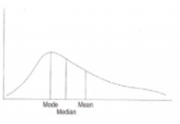
In case, a distribution is  skewed to the right, then  mean> median> mode.  

Generally, income distribution is skewed to the right where a large number of families have relatively  low income and a small number of families have extremely high income. In  such a case, the mean is pulled up by the extreme high incomes and the  relation among these three measures is as shown in Fig. Here, we find that  mean> median> mode.  

(ii) When a distribution is skewed to  

 the left, then mode> median>  

 mean. This is because here mean is  

 pulled down below the median  

 by extremely low values. This is 

41 

 shown as in the figure.  

(iii) Given the mean and median of a unimodal distribution, we can determine  whether it is skewed to the  right or left. When mean>  median, it is skewed to the  right; when median> mean, it  is skewed to the left. It may be noted that the median is always in the middle  between mean and mode.  

2.6 THE BEST MEASURE OF CENTRAL TENDENCY  At this stage, one may ask as to which of these three measures of central tendency the  best is. There is no simple answer to this question. It is because these three measures  are based upon different concepts. The arithmetic mean is the sum of the values  divided by the total number of observations in the series. The median is the value of  the middle observation that divides the series into two equal parts. Mode is the value  around which the observations tend to concentrate. As such, the use of a particular  measure will largely depend on the purpose of the study and the nature of the data;  For example, when we are interested in knowing the consumers preferences for  different brands of television sets or different kinds of advertising, the choice should  go in favour of mode. The use of mean and median would not be proper. However,  the median can sometimes be used in the case of qualitative data when such data can  be arranged in an ascending or descending order. Let us take another example.  Suppose we invite applications for a certain vacancy in our company. A large number  of candidates apply for that post. We are now interested to know as to which age or  age group has the largest concentration of applicants. Here, obviously the mode will  be the most appropriate choice. The arithmetic mean may not be appropriate as it may 

42 

be influenced by some extreme values. However, the mean happens to be the most  commonly used measure of central tendency as will be evident from the discussion in  the subsequent chapters.  

2.7 GEOMETRIC MEAN  

Apart from the three measures of central tendency as discussed above, there are two  other means that are used sometimes in business and economics. These are the  geometric mean and the harmonic mean. The geometric mean is more important than  the harmonic mean. We discuss below both these means. First, we take up the  geometric mean. Geometric mean is defined at the nth root of the product of n  observations of a distribution.  

Symbolically, GM = .... ..... ... _{1 2 n} n x x x If we have only two observations, say, 4 and  16 then GM = 4⋅16 = 64 = 8. Similarly, if there are three observations, then we  have to calculate the cube root of the product of these three observations; and so on.  When the number of items is large, it becomes extremely difficult to multiply the  numbers and to calculate the root. To simplify calculations, logarithms are used.  

Example 2.13: If we have to find out the geometric mean of 2, 4 and 8, then we find   ^{Log GM =} _n^x ∑ _i log 

Log2 + Log4 + Log8 

 ⁼ 3 

0.3010 + 0.6021+ 0.9031 

 ⁼ 3 

^1.8062 = 

 = 0.60206 

3 

 GM = Antilog 0.60206  

 = 4 

43 

When the data are given in the form of a frequency distribution, then the geometric  mean can be obtained by the formula:  

+ + + 

f . x f . x ... f . x _{l n n} 

log log log 

Log GM = _{f f fn} 

1 2 2 

∑ 

f x .log 

+ + 1 2 

.......... 

= _{f f fn} 

₁ + ₂ + 

Then, GM = Antilog n  

.......... 

The geometric mean is most suitable in the following three cases:  

1. Averaging rates of change.  

2. The compound interest formula.  

3. Discounting, capitalization.  

Example 2.14: A person has invested Rs 5,000 in the stock market. At the end of the  first year the amount has grown to Rs 6,250; he has had a 25 percent profit. If at the  end of the second year his principal has grown to Rs 8,750, the rate of increase is 40  percent for the year. What is the average rate of increase of his investment during the  two years?  

Solution:  

 GM = 1.25⋅1.40 = 1.75. = 1.323  

The average rate of increase in the value of investment is therefore 1.323 - 1 = 0.323,  which if multiplied by 100, gives the rate of increase as 32.3 percent.  

Example 2.15: We can also derive a compound interest formula from the above set of  data. This is shown below:  

Solution: Now, 1.25 x 1.40 = 1.75. This can be written as 1.75 = (1 + 0.323)².  Let P₂ = 1.75, P₀ = 1, and r = 0.323, then the above equation can be written as P₂ = (1  + r)² or P₂ = P₀ (1 + r)². 

44 

Where P2 is the value of investment at the end of the second year, P₀ is the initial  investment and r is the rate of increase in the two years. This, in fact, is the familiar  compound interest formula. This can be written in a generalised form as P_n = P₀(1 +  r)ⁿ. In our case Po is Rs 5,000 and the rate of increase in investment is 32.3 percent.  Let us apply this formula to ascertain the value of Pn, that is, investment at the end of  the second year.  

 P_n = 5,000 (1 + 0.323)² 

 = 5,000 x 1.75  

 = Rs 8,750  

It may be noted that in the above example, if the arithmetic mean is used, the resultant  ^{25 + 40}percent  

^{figure will be wrong. In this case, the average rate for the two years is} 2 ¹⁶⁵ x 5,000  

per year, which comes to 32.5. Applying this rate, we get P_n ⁼ 100 

 = Rs 8,250  

This is obviously wrong, as the figure should have been Rs 8,750.  

Example 2.16: An economy has grown at 5 percent in the first year, 6 percent in the  second year, 4.5 percent in the third year, 3 percent in the fourth year and 7.5 percent  in the fifth year. What is the average rate of growth of the economy during the five  years?  

Solution:  

Year Rate of Growth Value at the end of the Log x   ( percent) Year x (in Rs)  

1 5 105 2.02119  2 6 106 2.02531  3 4.5 104.5 2.01912  4 3 103 2.01284  5 7.5 107.5 2.03141   ∑ log X = 10.10987 

45 

_⎜^⎜_⎝^⎛∑_nlog x 

GM = Antilog _⎟^⎟_⎠⎞ 

10.10987 

= Antilog ^⎟_⎠^{⎞ ⎜}_⎝^⎛5 

= Antilog 2.021974  

= 105.19  

Hence, the average rate of growth during the five-year period is 105.19 - 100 = 5.19  percent per annum. In case of a simple arithmetic average, the corresponding rate of  growth would have been 5.2 percent per annum.  

2.7.1 DISCOUNTING  

The compound interest formula given above was  

P 

 P_n=P₀(1+r)ⁿ This can be written as P₀ = _n 

n 

_{(1+ )}  

r 

This may be expressed as follows:  

If the future income is P_n rupees and the present rate of interest is 100 r percent, then  the present value of P n rupees will be P₀ rupees. For example, if we have a machine  that has a life of 20 years and is expected to yield a net income of Rs 50,000 per year,  and at the end of 20 years it will be obsolete and cannot be used, then the machine's  present value is  

50,000 

50,000 

50,000 

50,000 

+ r⁺³ (1 ) 

₊+² (1 ) ⁿ (1 r) 

+ r^{+................. 20} (1 ) + r 

This process of ascertaining the present value of future income by using the interest  rate is known as discounting. 

In conclusion, it may be said that when there are extreme values in a series, geometric  mean should be used as it is much less affected by such values. The arithmetic mean  in such cases will give misleading results. 

46 

Before we close our discussion on the geometric mean, we should be aware of its  advantages and limitations.  

2.7.2 ADVANTAGES OF G. M.  

1. Geometric mean is based on each and every observation in the data set.  2. It is rigidly defined.  

3. It is more suitable while averaging ratios and percentages as also in calculating  growth rates.  

4. As compared to the arithmetic mean, it gives more weight to small values and  less weight to large values. As a result of this characteristic of the geometric  mean, it is generally less than the arithmetic mean. At times it may be equal to  the arithmetic mean.  

5. It is capable of algebraic manipulation. If the geometric mean has two or more  series is known along with their respective frequencies. Then a combined  geometric mean can be calculated by using the logarithms.  

2.7.3 LIMITATIONS OF G.M.  

1. As compared to the arithmetic mean, geometric mean is difficult to  understand.  

2. Both computation of the geometric mean and its interpretation are rather  difficult.  

3. When there is a negative item in a series or one or more observations have  zero value, then the geometric mean cannot be calculated.  

In view of the limitations mentioned above, the geometric mean is not frequently  used.  

2.8 HARMONIC MEAN 

47 

The harmonic mean is defined as the reciprocal of the arithmetic mean of the  reciprocals of individual observations. Symbolically,  

_ciprocal ⁿ ₌ ∑ 

^HM=_nx 

1/ 

Re 

1/ x₁ 1/ x₂ 1/ x₃ ... 1/ x_n 

+ + + + 

The calculation of harmonic mean becomes very tedious when a distribution has a  large number of observations. In the case of grouped data, the harmonic mean is  calculated by using the following formula:  

_{− ⎟}^⎟_⎠⎞ 

n 

 ^{HM = Reciprocal of} ∑

_⎜^⎜_⎝^⎛⋅ f 

1 

 or    

ⁱx 

ⁱ i 

1 

n 

_⎜^⎜_⎝^⎛⋅ 

_{− ⎟}^⎟_⎠⎞ 

n 

∑

f 

1 

ⁱx 

ⁱ i 

1 

Where n is the total number of observations.  

Here, each reciprocal of the original figure is weighted by the corresponding  frequency (f).  

The main advantage of the harmonic mean is that it is based on all observations in a  distribution and is amenable to further algebraic treatment. When we desire to give  greater weight to smaller observations and less weight to the larger observations, then  the use of harmonic mean will be more suitable. As against these advantages, there  are certain limitations of the harmonic mean. First, it is difficult to understand as well  as difficult to compute. Second, it cannot be calculated if any of the observations is  zero or negative. Third, it is only a summary figure, which may not be an actual  observation in the distribution.  

It is worth noting that the harmonic mean is always lower than the geometric mean,  which is lower than the arithmetic mean. This is because the harmonic mean assigns 

48 

lesser importance to higher values. Since the harmonic mean is based on reciprocals,  it becomes clear that as reciprocals of higher values are lower than those of lower  values, it is a lower average than the arithmetic mean as well as the geometric mean.  Example 2.17: Suppose we have three observations 4, 8 and 16. We are required to  ^{calculate the harmonic mean. Reciprocals of 4,8 and 16 are:} ₄^{1 ,}₈^{1 ,}₁₆¹ respectively  

n 

 Since HM = _{1/ x 1/ x 1/ x 1} + ₂ + ₃ 

3 

 = _{1/ 4 1/ 8 1/ 16} 

+ + 

3 

 = _{0.25 0.125 0.0625} 

+ + 

 = 6.857 approx.  

Example 2.18: Consider the following series:  

Class-interval 2-4 4-6 6-8 8-10  Frequency 20 40 30 10  

Solution:  

Let us set up the table as follows:  

Class-interval Mid-value Frequency Reciprocal of MV f x 1/x  

2-4 3 20 0.3333 6.6660  

4-6 5 40 0.2000 8.0000  

6-8 7 30 0.1429 4.2870  

8-10 9 10 0.1111 1.1111  

 Total 20.0641  

_⎜^⎜_⎝^⎛⋅ 

_{− ⎟}^⎟_⎠⎞ 

n 

∑ i f 

1 

= _nx 

1 

ⁱ i 

¹⁰⁰ = 4.984 approx. 

⁼ 20.0641 

49 

Example 2.19: In a small company, two typists are employed. Typist A types one  page in ten minutes while typist B takes twenty minutes for the same. (i) Both are  asked to type 10 pages. What is the average time taken for typing one page? (ii) Both  are asked to type for one hour. What is the average time taken by them for typing one  page?  

Solution: Here Q-(i) is on arithmetic mean while Q-(ii) is on harmonic mean.  (10 10) (20 20)(min ) 

⋅ + ⋅ 

 ^{(i) M =} 10 2( ) 

utes 

⋅ 

pages 

 = 15 minutes  ⋅ 

60 (min ) 

utes 

^{HM =} 60 /10 60 / 20( ) 

+ 

pages 

^{120 = =} ₊and 20 seconds.  

40 

= 13min utes 

120 60 20 

3 

Example 2.20: It takes ship A 10 days to cross the Pacific Ocean; ship B takes 15  days and ship C takes 20 days. (i) What is the average number of days taken by a ship  to cross the Pacific Ocean? (ii) What is the average number of days taken by a cargo  to cross the Pacific Ocean when the ships are hired for 60 days?  

Solution: Here again Q-(i) pertains to simple arithmetic mean while Q-(ii) is  concerned with the harmonic mean.  

10 +15 + ²⁰ = 15 days  

 ^{(i) M =} 3 

⋅ days 

60 3( ) _ 

^{(ii) HM =} 60 /10 60 /15 60 / 20 

+ + 

=  

180 

360 240 180 

+ +

60 

50 

= 13.8 days approx.  

2.9 QUADRATIC MEAN  

We have seen earlier that the geometric mean is the antilogarithm of the arithmetic  mean of the logarithms, and the harmonic mean is the reciprocal of the arithmetic  mean of the reciprocals. Likewise, the quadratic mean (Q) is the square root of the  arithmetic mean of the squares. Symbolically,  

2 

2 2 

₁ + + ...... + 

x x _n 

2 

^{Q =} n 

Instead of using original values, the quadratic mean can be used while averaging  deviations when the standard deviation is to be calculated. This will be used in the  next chapter on dispersion.  

2.9.1 Relative Position of Different Means  

The relative position of different means will always be:  

Q> x >G>H provided that all the individual observations in a series are positive and  all of them are not the same.  

2.9.2 Composite Average or Average of Means  

Sometimes, we may have to calculate an average of several averages. In such cases,  we should use the same method of averaging that was employed in calculating the  original averages. Thus, we should calculate the arithmetic mean of several values of  x, the geometric mean of several values of GM, and the harmonic mean of several  values of HM. It will be wrong if we use some other average in averaging of means.  

2.10 SUMMARY  

It is the most important objective of statistical analysis is to get one single value that  describes the characteristics of the entire mass of cumbersome data. Such a value is  finding out, which is known as central value to serve our purpose. 

51 

2.11 SELF-TEST QUESTIONS  

1. What are the desiderata (requirements) of a good average? Compare the mean,  the median and the mode in the light of these desiderata? Why averages are  called measures of central tendency?  

2. "Every average has its own peculiar characteristics. It is difficult to say which  average is the best." Explain with examples.  

3. What do you understand .by 'Central Tendency'? Under what conditions is the  median more suitable than other measures of central tendency?  

4. The average monthly salary paid to all employees in a company was Rs 8,000.  The average monthly salaries paid to male and female employees of the  company were Rs 10,600 and Rs 7,500 respectively. Find out the percentages  of males and females employed by the company.  

5. Calculate the arithmetic mean from the following data:  

Class 10-19 20-29 30-39 40-49 50-59 60-69 70-79 80-89  Frequency 2 4 9 11 12 6 4 2  6. Calculate the mean, median and mode from the following data:   Height in Inches Number of Persons  

62-63 2  

63-64 6  

64-65 14  

65-66 16  

66-67 8  

67-68 3  

68-69 1  

Total 50  

7. A number of particular articles have been classified according to their weights.  After drying for two weeks, the same articles have again been weighed and  similarly classified. It is known that the median weight in the first weighing 

52 

was 20.83 gm while in the second weighing it was 17.35 gm. Some  frequencies a and b in the first weighing and x and y in the second are missing.  It is known that a = 1/3x and b = 1/2 y. Find out the values of the missing  frequencies.  

Class Frequencies  

First Weighing Second Weighing  

0- 5 a z  

5-10 b y  

 10-15 11 40  

15-20 52 50  

20-25 75 30  

25-30 22 28  

8 Cities A, Band C are equidistant from each other. A motorist travels from A to  B at 30 km/h; from B to C at 40 km/h and from C to A at 50 km/h. Determine  his average speed for the entire trip.  

9 Calculate the harmonic mean from the following data:  

Class-Interval 2-4 4-6 6-8 8-10  Frequency 20 40 30 10  

10 A vehicle when climbing up a gradient, consumes petrol @ 8 km per litre.  While coming down it runs 12 km per litre. Find its average consumption for  to and fro travel between two places situated at the two ends of 25 Ian long  gradient. 

53 

2.12 Rest Karlo Thoda

WhatsApp Group pe baat karlo

 

This pdf is property of LaywerThink

And created by ShubhamYadav

 

COURSE: BUSINESS STATISTICS  

 

DISPERSION AND SKEWNESS 

OBJECTIVE: The objective of the present lesson is to impart the knowledge of  measures of dispersion and skewness and to enable the students to  distinguish between average, dispersion, skewness, moments and  kurtosis.  

STRUCTURE:  

3.1 Introduction  

3.2 Meaning and Definition of Dispersion  

3.3 Significance and Properties of Measuring Variation  

3.4 Measures of Dispersion  

3.5 Range  

3.6 Interquartile Range or Quartile Deviation  

3.7 Mean Deviation  

3.8 Standard Deviation  

3.9 Lorenz Curve  

3.10 Skewness: Meaning and Definitions  

3.11 Tests of Skewness  

3.12 Measures of Skewness  

3.13 Moments  

3.14 Kurtosis  

3.15 Summary  

3.16 Self-Test Questions  

3.17 surprise

3.1 INTRODUCTION  

In the previous chapter, we have explained the measures of central tendency. It may  be noted that these measures do not indicate the extent of dispersion or variability in a  distribution. The dispersion or variability provides us one more step in increasing our  understanding of the pattern of the data. Further, a high degree of uniformity (i.e. low  degree of dispersion) is a desirable quality. If in a business there is a high degree of  variability in the raw material, then it could not find mass production economical.  

55 

Suppose an investor is looking for a suitable equity share for investment. While  examining the movement of share prices, he should avoid those shares that are highly  fluctuating-having sometimes very high prices and at other times going very low.  Such extreme fluctuations mean that there is a high risk in the investment in shares.  The investor should, therefore, prefer those shares where risk is not so high.  

3.2 MEANING AND DEFINITIONS OF DISPERSION  The various measures of central value give us one single figure that represents the  entire data. But the average alone cannot adequately describe a set of observations,  unless all the observations are the same. It is necessary to describe the variability or  dispersion of the observations. In two or more distributions the central value may be  the same but still there can be wide disparities in the formation of distribution.  Measures of dispersion help us in studying this important characteristic of a  distribution.  

Some important definitions of dispersion are given below:  

1. "Dispersion is the measure of the variation of the items." -A.L. Bowley  2. "The degree to which numerical data tend to spread about an average value is  called the variation of dispersion of the data." -Spiegel  

3. Dispersion or spread is the degree of the scatter or variation of the variable  about a central value." -Brooks & Dick  4. "The measurement of the scatterness of the mass of figures in a series about an  

average is called measure of variation or dispersion." -Simpson & Kajka  It is clear from above that dispersion (also known as scatter, spread or variation)  measures the extent to which the items vary from some central value. Since measures  of dispersion give an average of the differences of various items from an average,  they are also called averages of the second order. An average is more meaningful  when it is examined in the light of dispersion. For example, if the average wage of the 

56 

workers of factory A is Rs. 3885 and that of factory B Rs. 3900, we cannot  necessarily conclude that the workers of factory B are better off because in factory B  there may be much greater dispersion in the distribution of wages. The study of  dispersion is of great significance in practice as could well be appreciated from the  following example:  

Series A Series B Series C  

100 100 1  

100 105 489  

100 102 2  

100 103 3  

100 90 5  

Total 500 500 500  

x ^{100 100 100}  

Since arithmetic mean is the same in all three series, one is likely to conclude that  these series are alike in  nature. But a close  examination shall reveal  that distributions differ  widely from one another.  In series A, (In Box-3.1)  each and every item is  perfectly represented by the  arithmetic mean or in other  words none of the items of  series A deviates from the 

57 

arithmetic mean and hence there is no dispersion. In series B, only one item is  perfectly represented by the arithmetic mean and the other items vary but the variation  is very small as compared to series C. In series C. not a single item is represented by  the arithmetic mean and the items vary widely from one another. In series C,  dispersion is much greater compared to series B. Similarly, we may have two groups  of labourers with the same mean salary and yet their distributions may differ widely.  The mean salary may not be so important a characteristic as the variation of the items  from the mean. To the student of social affairs the mean income is not so vitally  important as to know how this income is distributed. Are a large number receiving the  mean income or are there a few with enormous incomes and millions with incomes far  below the mean? The three figures given in Box 3.1 represent frequency distributions  with some of the characteristics. The two curves in diagram (a) represent two  distractions with the same mean X , but with different dispersions. The two curves in  (b) represent two distributions with the same dispersion but with unequal means X _l and X ₂, (c) represents two distributions with unequal dispersion. The measures of  central tendency are, therefore insufficient. They must be supported and supplemented  with other measures.  

In the present chapter, we shall be especially concerned with the measures of  variability or spread or dispersion. A measure of variation or dispersion is one that  measures the extent to which there are differences between individual observation and  some central or average value. In measuring variation we shall be interested in the  amount of the variation or its degree but not in the direction. For example, a measure  of 6 inches below the mean has just as much dispersion as a measure of six inches  above the mean. 

58 

Literally meaning of dispersion is ‘scatteredness’. Average or the measures of central  tendency gives us an idea of the concentration of the observations about the central  part of the distribution. If we know the average alone, we cannot form a complete idea  about the distribution. But with the help of dispersion, we have an idea about  homogeneity or heterogeneity of the distribution.  

3.3 SIGNIFICANCE AND PROPERTIES OF MEASURING  VARIATION  

 Measures of variation are needed for four basic purposes:  

1. Measures of variation point out as to how far an average is representative of  the mass. When dispersion is small, the average is a typical value in the sense  that it closely represents the individual value and it is reliable in the sense that  it is a good estimate of the average in the corresponding universe. On the other  hand, when dispersion is large, the average is not so typical, and unless the  sample is very large, the average may be quite unreliable.  

2. Another purpose of measuring dispersion is to determine nature and cause of  variation in order to control the variation itself. In matters of health variations  in body temperature, pulse beat and blood pressure are the basic guides to  diagnosis. Prescribed treatment is designed to control their variation. In  industrial production efficient operation requires control of quality variation  the causes of which are sought through inspection is basic to the control of  causes of variation. In social sciences a special problem requiring the  measurement of variability is the measurement of "inequality" of the  distribution of income or wealth etc.  

3. Measures of dispersion enable a comparison to be made of two or more series  with regard to their variability. The study of variation may also be looked 

59 

upon as a means of determining uniformity of consistency. A high degree of  variation would mean little uniformity or consistency whereas a low degree of  variation would mean great uniformity or consistency.  

4. Many powerful analytical tools in statistics such as correlation analysis. the  testing of hypothesis, analysis of variance, the statistical quality control,  regression analysis is based on measures of variation of one kind or another.  A good measure of dispersion should possess the following properties  

1. It should be simple to understand.  

2. It should be easy to compute.  

3. It should be rigidly defined.  

4. It should be based on each and every item of the distribution.  

5. It should be amenable to further algebraic treatment.  

6. It should have sampling stability.  

7. Extreme items should not unduly affect it. 

3.4 MEAURES OF DISPERSION  

There are five measures of dispersion: Range, Inter-quartile range or Quartile  Deviation, Mean deviation, Standard Deviation, and Lorenz curve. Among them, the  first four are mathematical methods and the last one is the graphical method. These  are discussed in the ensuing paragraphs with suitable examples.  

3.5 RANGE  

The simplest measure of dispersion is the range, which is the difference between the  maximum value and the minimum value of data.  

Example 3.1: Find the range for the following three sets of data:  

Set 1: 05 15 15 05 15 05 15 15 15 15  Set 2: 8 7 15 11 12 5 13 11 15 9 

60 

Set 3: 5 5 5 5 5 5 5 5 5 5  Solution: In each of these three sets, the highest number is 15 and the lowest number  is 5. Since the range is the difference between the maximum value and the minimum  value of the data, it is 10 in each case. But the range fails to give any idea about the  dispersal or spread of the series between the highest and the lowest value. This  becomes evident from the above data.  

In a frequency distribution, range is calculated by taking the difference between the  upper limit of the highest class and the lower limit of the lowest class.  Example 3.2: Find the range for the following frequency distribution:  

Size of Item Frequency  

20- 40 7  

40- 60 11  

60- 80 30  

80-100 17  

100-120 5  

Total 70  

Solution: Here, the upper limit of the highest class is 120 and the lower limit of the  lowest class is 20. Hence, the range is 120 - 20 = 100. Note that the range is not  influenced by the frequencies. Symbolically, the range is calculated b the formula L -  S, where L is the largest value and S is the smallest value in a distribution. The  coefficient of range is calculated by the formula: (L-S)/ (L+S). This is the relative  measure. The coefficient of the range in respect of the earlier example having three  sets of data is: 0.5.The coefficient of range is more appropriate for purposes of  comparison as will be evident from the following example:  

Example 3.3: Calculate the coefficient of range separately for the two sets of data  given below:  

Set 1 8 10 20 9 15 10 13 28  Set 2 30 35 42 50 32 49 39 33 

61 

Solution: It can be seen that the range in both the sets of data is the same:  Set 1 28 - 8 = 20  

Set 2 50 - 30 = 20  

Coefficient of range in Set 1 is:  

28 – 8 = 0.55  

28+8  

Coefficient of range in set 2 is:  

50 – 30  50 +30  

= 0.25 

3.5.1 LIMITATIONS OF RANGE 

 There are some limitations of range, which are as follows:  

1. It is based only on two items and does not cover all the items in a distribution.  2. It is subject to wide fluctuations from sample to sample based on the same  population.  

3. It fails to give any idea about the pattern of distribution. This was evident from  the data given in Examples 1 and 3.  

4. Finally, in the case of open-ended distributions, it is not possible to compute  the range.  

Despite these limitations of the range, it is mainly used in situations where one wants  to quickly have some idea of the variability or' a set of data. When the sample size is  very small, the range is considered quite adequate measure of the variability. Thus, it  is widely used in quality control where a continuous check on the variability of raw  materials or finished products is needed. The range is also a suitable measure in  weather forecast. The meteorological department uses the range by giving the  maximum and the minimum temperatures. This information is quite useful to the  common man, as he can know the extent of possible variation in the temperature on a  particular day.  

62 

3.6 INTERQUARTILE RANGE OR QUARTILE DEVIATION  The interquartile range or the quartile deviation is a better measure of variation in a  distribution than the range. Here, avoiding the 25 percent of the distribution at both  the ends uses the middle 50 percent of the distribution. In other words, the  interquartile range denotes the difference between the third quartile and the first  quartile.  

Symbolically, interquartile range = Q₃- Q_l 

Many times the interquartile range is reduced in the form of semi-interquartile range  or quartile deviation as shown below:  

Semi interquartile range or Quartile deviation = (Q₃ – Q_l)/2  

When quartile deviation is small, it means that there is a small deviation in the central  50 percent items. In contrast, if the quartile deviation is high, it shows that the central  50 percent items have a large variation. It may be noted that in a symmetrical  distribution, the two quartiles, that is, Q3 and QI are equidistant from the median.  Symbolically,  

 M-Q_I = Q₃-M  

However, this is seldom the case as most of the business and economic data are  asymmetrical. But, one can assume that approximately 50 percent of the observations  are contained in the interquartile range. It may be noted that interquartile range or the  quartile deviation is an absolute measure of dispersion. It can be changed into a  relative measure of dispersion as follows:  

 Coefficient of QD = 

Q₃ –Q₁ Q₃ +Q₁ 

The computation of a quartile deviation is very simple, involving the computation of  upper and lower quartiles. As the computation of the two quartiles has already been  explained in the preceding chapter, it is not attempted here.  

63 

 3.6.1 MERITS OF QUARTILE DEVIATION  

 The following merits are entertained by quartile deviation:  

1. As compared to range, it is considered a superior measure of dispersion.  2. In the case of open-ended distribution, it is quite suitable.  

3. Since it is not influenced by the extreme values in a distribution, it is  particularly suitable in highly skewed or erratic distributions.  

3.6.2 LIMITATIONS OF QUARTILE DEVIATION 

1. Like the range, it fails to cover all the items in a distribution.  

2. It is not amenable to mathematical manipulation.  

3. It varies widely from sample to sample based on the same population.  4. Since it is a positional average, it is not considered as a measure of dispersion.  It merely shows a distance on scale and not a scatter around an average.  In view of the above-mentioned limitations, the interquartile range or the quartile  deviation has a limited practical utility.  

3.7 MEAN DEVIATION  

The mean deviation is also known as the average deviation. As the name implies, it is  the average of absolute amounts by which the individual items deviate from the mean.  Since the positive deviations from the mean are equal to the negative deviations,  while computing the mean deviation, we ignore positive and negative signs.  Symbolically,  

∑^{| x |} Where MD = mean deviation, |x| = deviation of an item  MD = _n 

from the mean ignoring positive and negative signs, n = the total number of  observations. 

64 

 Example 3.4:  

Size of Item Frequency  

2-4 20  

4-6 40  

6-8 30  

8-10 10  

Solution: 

^{Size of Item Mid-points (m) Frequency (f) fm} d from x ^{f |d|}  

2-4 3 20 60 -2.6 52  

4-6 5 40 200 -0.6 24  

6-8 7 30 210 1.4 42  

8-10 9 10 90 3.4 34  

Total 100 560 152  

⁵⁶⁰ _{= =} ∑_nfm 

x = 5.6 

100 

^{| | 152} _{= =} ∑_nf d 

 MD ( x ) = 1.52 

100 

3.7.1 MERITS OF MEAN DEVIATION 

1. A major advantage of mean deviation is that it is simple to understand and  easy to calculate.  

2. It takes into consideration each and every item in the distribution. As a result,  a change in the value of any item will have its effect on the magnitude of mean  deviation.  

3. The values of extreme items have less effect on the value of the mean  deviation.  

4. As deviations are taken from a central value, it is possible to have meaningful  comparisons of the formation of different distributions.  

3.7.2 LIMITATIONS OF MEAN DEVIATION 

1. It is not capable of further algebraic treatment. 

65 

2. At times it may fail to give accurate results. The mean deviation gives best  results when deviations are taken from the median instead of from the mean.  But in a series, which has wide variations in the items, median is not a  satisfactory measure.  

3. Strictly on mathematical considerations, the method is wrong as it ignores the  algebraic signs when the deviations are taken from the mean.  

In view of these limitations, it is seldom used in business studies. A better measure  known as the standard deviation is more frequently used.  

3.8 STANDARD DEVIATION  

The standard deviation is similar to the mean deviation in that here too the deviations  are measured from the mean. At the same time, the standard deviation is preferred to  the mean deviation or the quartile deviation or the range because it has desirable  mathematical properties.  

Before defining the concept of the standard deviation, we introduce another concept  viz. variance.  

Example 3.5:  

X X-μ (X-μ)² 

20 20-18=12 4  

15 15-18= -3 9  

19 19-18 = 1 1  

24 24-18 = 6 36  

16 16-18 = -2 4  

14 14-18 = -4 16  

108 Total 70  

Solution:  

^{Mean =} ₆¹⁰⁸ = 18 

66 

The second column shows the deviations from the mean. The third or the last column  shows the squared deviations, the sum of which is 70. The arithmetic mean of the  squared deviations is:  

∑ ^{x − 2} 

 ( ) 

N 

^μ = 70/6=11.67 approx.  

This mean of the squared deviations is known as the variance. It may be noted that  this variance is described by different terms that are used interchangeably: the  variance of the distribution X; the variance of X; the variance of the distribution; and  just simply, the variance.  

∑ ^{x − 2} 

_{Symbolically, Var (X) =} ( ) 

μ 

N 

^x ∑ _i ⁻ =² 

_{It is also written as} ( ) 

σ 

₂ μ N 

Where σ² (called sigma squared) is used to denote the variance.  

Although the variance is a measure of dispersion, the unit of its measurement is  (points). If a distribution relates to income of families then the variance is (Rs)² and  not rupees. Similarly, if another distribution pertains to marks of students, then the  unit of variance is (marks)². To overcome this inadequacy, the square root of variance  is taken, which yields a better measure of dispersion known as the standard deviation.  Taking our earlier example of individual observations, we take the square root of the  variance  

 SD or σ = Variance = 11 = 3.42 points .67 

^x ∑ _i − ² μ 

Symbolically, σ = ^{( )} 

N 

In applied Statistics, the standard deviation is more frequently used than the variance.  This can also be written as: 

67 

σ =  

∑ _i∑₋2 

( ) 

x 

x ⁱ 

2 

N 

N 

We use this formula to calculate the standard deviation from the individual  observations given earlier.  

Example 7.6:  

X X² 

20 400  

15 225  

19 361  

24 576  

16 256  

14 196  

108 2014  

Solution:  

∑ ^x_i ⁼ ∑ ^{= N = 6}  

2 

2014 x 108 _i 

( ) 

¹⁰⁸ 2014² 

¹¹⁶⁶⁴ 2014 − 

σ =  

− 

6 

6 

 ^{Or, σ =} ₆6 

12084 −11664 

σ ⁼ ₆6 

420 

 ^{Or, σ =} ₆6 

 σ =  

⁷⁰ Or, σ = 11.67  6 

 σ = 3.42  

Example 3.7:  

The following distribution relating to marks obtained by students in an examination:  

Marks Number of Students  

0- 10 1  

10- 20 3  

20- 30 6  

30- 40 10  

40- 50 12  

50- 60 11 

68 

60- 70 6  

70- 80 3  

80- 90 2  

90-100 1  

Solution:  

Marks Frequency (f) Mid-points Deviations (d)/10=d’ Fd’ fd'² 

0- 10 1 5 -5 -5 25  

10- 20 3 15 -4 -12 48  

20- 30 6 25 -3 -18 54  

30- 40 10 35 -2 -20 40  

40- 50 12 45 -1 -12 12  

50- 60 11 55 0 0 0  

60- 70 6 65 1 6 6  

70- 80 3 75 2 6 12  

80- 90 2 85 3 6 18  

90-100 1 95 4 4 16  

Total 55 Total -45 231  

In the case of frequency distribution where the individual values are not known, we  use the midpoints of the class intervals. Thus, the formula used for calculating  the standard deviation is as given below:  

K 

∑ i 

( ) 

2 

σ =  

i 

= 

− 

1 

fi m 

μ 

N 

Where m_i is the mid-point of the class intervals μ is the mean of the distribution, fi is  the frequency of each class; N is the total number of frequency and K is the number of  classes. This formula requires that the mean μ be calculated and that deviations (m_i -  μ) be obtained for each class. To avoid this inconvenience, the above formula can be  modified as:  

_i ^⎟_⎠^{⎞ ⎜}_⎝^⎛ ∑ ∑ _{=1 =1} 

K 

2 

K 

fid fd 

i 

σ = _N 

i 

i 

Where C is the class interval: f_i is the frequency of the ith class and d_i is the deviation  of the of item from an assumed origin; and N is the total number of observations.   Applying this formula for the table given earlier,  

σ = 

2 

²³¹ 10 ^⎟_⎠^{⎞ ⎜}_⎝⎛ ⁻ −45 

55 

55 

69 

 =10 4.2 − 0.669421 

 =18.8 marks  

When it becomes clear that the actual mean would turn out to be in fraction,  calculating deviations from the mean would be too cumbersome. In such cases,  an assumed mean is used and the deviations from it are calculated. While mid point of any class can be taken as an assumed mean, it is advisable to choose  the mid-point of that class that would make calculations least cumbersome.  Guided by this consideration, in Example 3.7 we have decided to choose 55 as  the mid-point and, accordingly, deviations have been taken from it. It will be  seen from the calculations that they are considerably simplified.  

3.8.1 USES OF THE STANDARD DEVIATION  

The standard deviation is a frequently used measure of dispersion. It enables us to  determine as to how far individual items in a distribution deviate from its mean. In a  symmetrical, bell-shaped curve:  

(i) About 68 percent of the values in the population fall within: + 1 standard  deviation from the mean.  

(ii) About 95 percent of the values will fall within +2 standard deviations from the  mean.  

(iii) About 99 percent of the values will fall within + 3 standard deviations from  the mean.  

The standard deviation is an absolute measure of dispersion as it measures variation in  the same units as the original data. As such, it cannot be a suitable measure while  comparing two or more distributions. For this purpose, we should use a relative  measure of dispersion. One such measure of relative dispersion is the coefficient of  variation, which relates the standard deviation and the mean such that the standard  deviation is expressed as a percentage of mean. Thus, the specific unit in which the  standard deviation is measured is done away with and the new unit becomes percent. 

70 

σ 

Symbolically, CV (coefficient of variation) = x 100 

μ 

Example 3.8: In a small business firm, two typists are employed-typist A and typist  B. Typist A types out, on an average, 30 pages per day with a standard deviation of 6.  Typist B, on an average, types out 45 pages with a standard deviation of 10. Which  typist shows greater consistency in his output?  

^σ A = 

Solution: Coefficient of variation for x 100 

μ 

⁶ A = 

 Or x 100 

30 

Or 20% and  

^σ B = 

Coefficient of variation for x 100 

μ 

¹⁰ B = 

 x 100 

45 

or 22.2 %  

These calculations clearly indicate that although typist B types out more pages, there  is a greater variation in his output as compared to that of typist A. We can say this in a  different way: Though typist A's daily output is much less, he is more consistent than  typist B. The usefulness of the coefficient of variation becomes clear in comparing  two groups of data having different means, as has been the case in the above example.  

3.8.2 STANDARDISED VARIABLE, STANDARD SCORES The variable Z = (x - x )/s or (x - μ)/μ, which measures the deviation from the mean  in units of the standard deviation, is called a standardised variable. Since both the  numerator and the denominator are in the same units, a standardised variable is  independent of units used. If deviations from the mean are given in units of the  standard deviation, they are said to be expressed in standard units or standard scores. 

71 

Through this concept of standardised variable, proper comparisons can be made  between individual observations belonging to two different distributions whose  compositions differ.  

Example 3.9: A student has scored 68 marks in Statistics for which the average  marks were 60 and the standard deviation was 10. In the paper on Marketing, he  scored 74 marks for which the average marks were 68 and the standard deviation was  15. In which paper, Statistics or Marketing, was his relative standing higher?  

Solution: The standardised variable Z = (x - x ) ⎟ s measures the deviation of x from  the mean x in terms of standard deviation s. For Statistics, Z = (68 - 60) ⎟ 10 = 0.8   For Marketing, Z = (74 - 68) ⎟ 15 = 0.4  

Since the standard score is 0.8 in Statistics as compared to 0.4 in Marketing, his  relative standing was higher in Statistics.  

Example 3.10: Convert the set of numbers 6, 7, 5, 10 and 12 into standard scores:  Solution:  

X ^X2 

6 36  

7 49  

5 25  

10 100  

12 144  

∑ ^{X = 40 2} 

∑^{X = 354}  

^{x =} ∑^{x ⎟ N = 40 ⎟ 5 = 8} 

∑^x ∑₋2 

σ =  

2 

 or, σ =  

( ) 

X 

N 

( ) 

⁴⁰ 354² 

− 

5 

5 

N 

^{354 − 320} = 2.61 approx.  =₅ 

72 

x x _{= -0.77 (Standard score)}  

^{6 − 8} ₌ −_σ 

 ^{Z =}2.61 

Applying this formula to other values:  

^{7 − 8} = -0.38  

⁽ⁱ⁾ 2.61 

^{5 − 8} = -1.15  

⁽ⁱⁱ⁾ 2.61 

^{10 − 8} = 0.77  

⁽ⁱⁱⁱ⁾ 2.61 

^{12 − 8} = 1.53  

^(iv) 2.61 

Thus the standard scores for 6,7,5,10 and 12 are -0.77, -0.38, -1.15, 0.77 and 1.53,  respectively.  

3.9 LORENZ CURVE  

This measure of dispersion is graphical. It is known as the Lorenz curve named after  Dr. Max Lorenz. It is generally used to show the extent of concentration of income  and wealth. The steps involved in plotting the Lorenz curve are:  

1. Convert a frequency distribution into a cumulative frequency table.  2. Calculate percentage for each item taking the total equal to 100.  3. Choose a suitable scale and plot the cumulative percentages of the persons and  

income. Use the horizontal axis of X to depict percentages of persons and the  vertical axis of Y to depict percent ages of income.  

4. Show the line of equal distribution, which will join 0 of X-axis with 100 of Y axis.  

5. The curve obtained in (3) above can now be compared with the straight line of  equal distribution obtained in (4) above. If the Lorenz curve is close to the line  of equal distribution, then it implies that the dispersion is much less. If, on the 

73 

contrary, the Lorenz curve is farther away from the line of equal distribution,  it implies that the dispersion is considerable.  

The Lorenz curve is a simple graphical device to show the disparities of distribution  in any phenomenon. It is, used in business and economics to represent inequalities in  income, wealth, production, savings, and so on.  

Figure 3.1 shows two Lorenz curves by way of illustration. The straight line AB is a  line of equal distribution, whereas AEB shows complete inequality. Curve ACB and  curve ADB are the Lorenz curves.  

sry ye mila nahi

Figure 3.1: Lorenz Curve  

As curve ACB is nearer to the line of equal distribution, it has more equitable  distribution of income than curve ADB. Assuming that these two curves are for the  same company, this may be interpreted in a different manner. Prior to taxation, the  curve ADB showed greater inequality in the income of its employees. After the  taxation, the company’s data resulted into ACB curve, which is closer to the line of  equal distribution. In other words, as a result of taxation, the inequality has reduced.  

3.10 SKEWNESS: MEANING AND DEFINITIONS  

In the above paragraphs, we have discussed frequency distributions in detail. It may  be repeated here that frequency distributions differ in three ways: Average value,  Variability or dispersion, and Shape. Since the first two, that is, average value and 

74 

variability or dispersion have already been discussed in previous chapters, here our  main spotlight will be on the shape of frequency distribution. Generally, there are two  comparable characteristics called skewness and kurtosis that help us to understand a  distribution. Two distributions may have the same mean and standard deviation but  may differ widely in their overall appearance as can be seen from the following:  

In both these distributions the value of  

mean and standard deviation is the same  

( X = 15, σ = 5). But it does not imply  

that the distributions are alike in nature.  

The distribution on the left-hand side is  

a symmetrical one whereas the distribution on the right-hand side is symmetrical or  skewed. Measures of skewness help us to distinguish between different types of  distributions.  

Some important definitions of skewness are as follows:  

1. "When a series is not symmetrical it is said to be asymmetrical or skewed."  -Croxton & Cowden.  2. "Skewness refers to the asymmetry or lack of symmetry in the shape of a  frequency distribution." -Morris Hamburg.  3. "Measures of skewness tell us the direction and the extent of skewness. In  symmetrical distribution the mean, median and mode are identical. The more  the mean moves away from the mode, the larger the asymmetry or skewness."  -Simpson & Kalka  4. "A distribution is said to be 'skewed' when the mean and the median fall at  different points in the distribution, and the balance (or centre of gravity) is  shifted to one side or the other-to left or right." -Garrett 

75 

The above definitions show that the term 'skewness' refers to lack of symmetry" i.e.,  when a distribution is not symmetrical (or is asymmetrical) it is called a skewed  distribution.  

The concept of skewness will be clear from the following three diagrams showing a  symmetrical distribution. a positively skewed distribution and a negatively skewed  distribution.  

1. Symmetrical Distribution. It is clear from the diagram (a) that in a sym metrical distribution the values of mean, median and mode coincide. The  spread of the frequencies is the same on  

both sides of the centre point of the curve.  

2. Asymmetrical Distribution. A  

distribution, which is not symmetrical, is  

called a skewed distribution and such a  

distribution could either be positively  

skewed or negatively skewed as would be  

clear from the diagrams (b) and (c).  

3. Positively Skewed Distribution. In the  

positively skewed distribution the value of  

the mean is maximum and that of mode least-the median lies in between the  two as is clear from the diagram (b).  

4. Negatively Skewed Distribution. The following is the shape of negatively  skewed distribution. In a negatively skewed distribution the value of mode is  maximum and that of mean least-the median lies in between the two. In the  positively skewed distribution the frequencies are spread out over a greater 

76 

range of values on the high-value end of the curve (the right-hand side) than  they are on the low-value end. In the negatively skewed distribution the  position is reversed, i.e. the excess tail is on the left-hand side. It should be  noted that in moderately symmetrical distributions the interval between the  mean and the median is approximately one-third of the interval between the  mean and the mode. It is this relationship, which provides a means of  measuring the degree of skewness.  

3.11 TESTS OF SKEWNESS  

In order to ascertain whether a distribution is skewed or not the following tests may  be applied. Skewness is present if:  

1. The values of mean, median and mode do not coincide.  

2. When the data are plotted on a graph they do not give the normal bell shaped form i.e. when cut along a vertical line through the centre the two  halves are not equal.  

3. The sum of the positive deviations from the median is not equal to the sum  of the negative deviations.  

4. Quartiles are not equidistant from the median.  

5. Frequencies are not equally distributed at points of equal deviation from  the mode.  

On the contrary, when skewness is absent, i.e. in case of a symmetrical distribution,  the following conditions are satisfied:  

1. The values of mean, median and mode coincide.  

2. Data when plotted on a graph give the normal bell-shaped form.  3. Sum of the positive deviations from the median is equal to the sum of the  negative deviations. 

77 

4. Quartiles are equidistant from the median.  

5. Frequencies are equally distributed at points of equal deviations from the  mode.  

3.12 MEASURES OF SKEWNESS  

There are four measures of skewness, each divided into absolute and relative  measures. The relative measure is known as the coefficient of skewness and is more  frequently used than the absolute measure of skewness. Further, when a comparison  between two or more distributions is involved, it is the relative measure of skewness,  which is used. The measures of skewness are: (i) Karl Pearson's measure, (ii)  Bowley’s measure, (iii) Kelly’s measure, and (iv) Moment’s measure. These  measures are discussed briefly below:  

3.12.1 KARL PEARON’S MEASURE  

The formula for measuring skewness as given by Karl Pearson is as follows:   Skewness = Mean - Mode  

Coefficient of skewness =  

Mean – Mode 

Standard Deviation 

In case the mode is indeterminate, the coefficient of skewness is:  

Sk_p =  Sk_p =  

Mean - (3 Median - 2 Mean) Standard deviation 

3(Mean - Median) 

Standard deviation  

 Now this formula is equal to the earlier one.  

3(Mean - Median) 

  

Standard deviation  

Or 3 Mean - 3 Median = Mean - Mode  Or Mode = Mean - 3 Mean + 3 Median  Or Mode = 3 Median - 2 Mean  

Mean - Mode 

Standard deviation 

The direction of skewness is determined by ascertaining whether the mean is greater  than the mode or less than the mode. If it is greater than the mode, then skewness is  

78 

positive. But when the mean is less than the mode, it is negative. The difference  between the mean and mode indicates the extent of departure from symmetry. It is  measured in standard deviation units, which provide a measure independent of the  unit of measurement. It may be recalled that this observation was made in the  preceding chapter while discussing standard deviation. The value of coefficient of  skewness is zero, when the distribution is symmetrical. Normally, this coefficient of  skewness lies between +1. If the mean is greater than the mode, then the coefficient of  skewness will be positive, otherwise negative.  

Example 3.11: Given the following data, calculate the Karl Pearson's coefficient of  skewness: ∑x = 452 ∑x²= 24270 Mode = 43.7 and N = 10  Solution:  

Pearson's coefficient of skewness is:  

 Sk_P =  

Mean - Mode 

Standard deviation  

⁴⁵² _{= =} ∑_N^X  

 Mean ( x )= _45.2 10 

_⎜^⎜_⎝^⎛ ₌ ∑ ₋ ∑_Nx 

 SD _{( )2} ²_⎟^⎟_⎠⎞ 

_⎜^⎜_⎝^⎛ ₌ ∑ ₋ ∑_Nx 

^x σ ( )^{2 2}_⎟^⎟_⎠⎞ 

N 

2 

^x σ N 

^{24270 ⎟}_⎠^{⎞ ⎜}_⎝^⎛ σ _{= −} 2427 (45.2) 19.59 ² 

( ) 

10 

452 10 

= − = 

Applying the values of mean, mode and standard deviation in the above formula,  

 Sk_p =  =0.08  

45.2 – 43.7  19.59 

This shows that there is a positive skewness though the extent of skewness is  marginal.  

Example 3.12: From the following data, calculate the measure of skewness using the  mean, median and standard deviation:  

X 10 - 20 20 - 30 30 - 40 40 - 50 50-60 60 - 70 70 - 80  f 18 30 40 55 38 20 16  

79 

Solution: 

x MVx d_x f fd_x fd_X² cf  

10 - 20 15 -3 18 -54 162 18  

20 - 30 25 -2 30 -60 120 48  

30 - 40 35 -1 40 -40 40 88  

40-50 45=a 0 55 0 0 143  

50 - 60 55 1 38 38 38 181  

60 - 70 65 2 20 40 80 201  

70 - 80 75 3 16 48 144 217  

 Total 217 -28 584  

a = Assumed mean = 45, cf = Cumulative frequency, dx = Deviation from assumed  mean, and i = 10  

x = a _{+ ⋅} ∑ 

fdx N 

i 

²⁸ = 45 − ⋅ = 

217 

10 43.71 l l ₋ ⁻ + 

Median= l₁ ( ) 

^{2 1} m c 

f 

1 

Where m = (N + 1)/2^th item  

= (217 + 1)/2 = 109^th item  

^{50 40} _{40 −} ⁻ = − 

 Median ^{(109 88)} 55 

¹⁰ = 40 + ⋅ 

55 

 = 43.82  

21 

∑ 

⁵⁸⁴ 10^{2 2 2}⎟ ⋅ ⁻_∑∑ 

_⎜^⎜_⎝⎛ 

fd_{x x} fd 

^{⎞ ⎜}_⎝⎛ ^{− ⋅ = −} _⎟^⎟_⎠⎞ 28 

SD = ₁₀ 

∑ 

f 

f 

217 

217 

⎠ 

 = 2.69 - 0.016 ⋅10 = 16.4  Skewness = 3 (Mean - Median)   = 3 (43.71 - 43.82)   = 3 x -0.011 

80